YTjnti

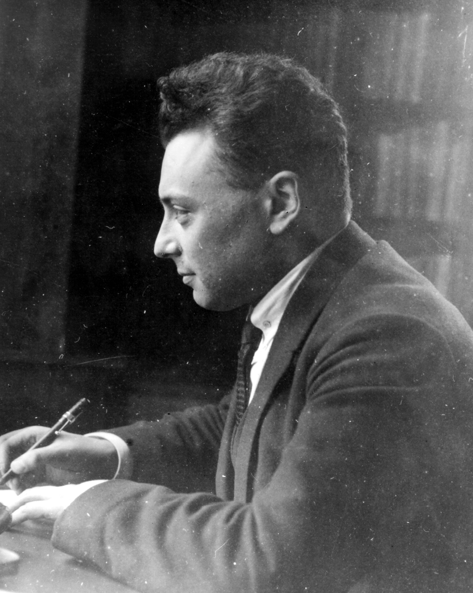
Wolfgang Pauli (1900–1958), ca. 1924. Pauli received the Nobel Prize in physics in 1945, nominated by Albert Einstein, for the Pauli exclusion principle.

In mathematical physics and mathematics, the Pauli matrices are a set of three $2 \times 2$ complex matrices which are Hermitian and unitary.^[1] Usually indicated by the Greek letter sigma ( $σ$ ), they are occasionally denoted by tau ( $τ$ ) when used in connection with isospin symmetries. They are

beginalignedsigma _1=sigma _x&=beginpmatrix0&1\1&0endpmatrix\sigma _2=sigma _y&=beginpmatrix0&-i\i&0endpmatrix\sigma _3=sigma _z&=beginpmatrix1&0\0&-1endpmatrix,.endaligned

These matrices are named after the physicist Wolfgang Pauli. In quantum mechanics, they occur in the Pauli equation which takes into account the interaction of the spin of a particle with an external electromagnetic field.

Each Pauli matrix is Hermitian, and together with the identity matrix $I$ (sometimes considered as the zeroth Pauli matrix $σ 0$ ), the Pauli matrices (multiplied by real coefficients) form a basis for the vector space of $2 \times 2$ Hermitian matrices.

Hermitian operators represent observables, so the Pauli matrices span the space of observables of the $2$ -dimensional complex Hilbert space. In the context of Pauli's work, $σ k$ represents the observable corresponding to spin along the $k$ th coordinate axis in three-dimensional Euclidean space $ℝ 3$ .

The Pauli matrices (after multiplication by $i$ to make them anti-Hermitian), also generate transformations in the sense of Lie algebras: the matrices $iσ 1, iσ 2, iσ 3$ form a basis for $mathfrak su(2)$ , which exponentiates to the special unitary group SU(2).^{[nb 1]} The algebra generated by the three matrices $σ 1, σ 2, σ 3$ is isomorphic to the Clifford algebra of $ℝ 3$ .

1 Algebraic properties
- 1.1 Eigenvectors and eigenvalues
- 1.2 Pauli vector
- 1.3 Commutation relations
- 1.4 Relation to dot and cross product
- 1.5 Some trace relations
- 1.6 Exponential of a Pauli vector
  - 1.6.1 The group composition law of SU(2)
  - 1.6.2 Adjoint action
- 1.7 Completeness relation
- 1.8 Relation with the permutation operator

2 SU(2)
- 2.1 SO(3)
- 2.2 Quaternions

3 Physics
- 3.1 Classical mechanics
- 3.2 Quantum mechanics
- 3.3 Relativistic quantum mechanics
- 3.4 Quantum information

4 See also

5 Remarks

6 Notes

7 References

Algebraic properties

All three of the Pauli matrices can be compacted into a single expression:

sigma _a=beginpmatrixdelta _a3&delta _a1-idelta _a2\delta _a1+idelta _a2&-delta _a3endpmatrix

where $i = \sqrt -1$ is the imaginary unit, and $δ ab$ is the Kronecker delta, which equals +1 if $a = b$ and 0 otherwise. This expression is useful for "selecting" any one of the matrices numerically by substituting values of $a = 1, 2, 3$ , in turn useful when any of the matrices (but no particular one) is to be used in algebraic manipulations.

The matrices are involutory:

sigma_1^2 = sigma_2^2 = sigma_3^2 = -isigma_1 sigma_2 sigma_3 = beginpmatrix 1&0\0&1endpmatrix = I

where $I$ is the identity matrix.

The determinants and traces of the Pauli matrices are:

beginaligneddet sigma _i&=-1,\operatorname Trsigma _i&=0.endaligned

From above we can deduce that the eigenvalues of each $σ i$ are $\pm1$ .

Together with the $2 \times 2$ identity matrix $I$ (sometimes written as $σ 0$ ), the Pauli matrices form an orthogonal basis, in the sense of Hilbert–Schmidt, for the real Hilbert space of $2 \times 2$ complex Hermitian matrices, or the complex Hilbert space of all $2 \times 2$ matrices.

Eigenvectors and eigenvalues

Each of the (Hermitian) Pauli matrices has two eigenvalues, $+1$ and $-1$ . The corresponding normalized eigenvectors are:

displaystyle beginaligned&psi _x+=frac 1sqrt 2beginpmatrix1\1endpmatrix,&&psi _x-=frac 1sqrt 2beginpmatrix1\-1endpmatrix,\&psi _y+=frac 1sqrt 2beginpmatrix1\iendpmatrix,&&psi _y-=frac 1sqrt 2beginpmatrix1\-iendpmatrix,\&psi _z+=beginpmatrix1\0endpmatrix,&&psi _z-=beginpmatrix0\1endpmatrix.endaligned

Pauli vector

The Pauli vector is defined by^{[nb 2]}

displaystyle vec sigma =sigma _1hat x+sigma _2hat y+sigma _3hat z

and provides a mapping mechanism from a vector basis to a Pauli matrix basis^[2] as follows,

beginalign

using the summation convention. Further,

det vec acdot vec sigma =-vec acdot vec a=-|vec a|^2,

its eigenvalues being $vec a$ , and moreover (see completeness, below)

displaystyle frac 12mathrm tr [(vec acdot vec sigma )vec sigma ]=vec a~.

Its (unnormalized) eigenvectors are
$displaystyle psi _+=\a_1+ia_2endpmatrix;qquad psi _-=beginpmatrixia_2-a_1\a_3+.$

Commutation relations

The Pauli matrices obey the following commutation relations:

[sigma_a, sigma_b] = 2 i varepsilon_a b c,sigma_c , ,

and anticommutation relations:

sigma_a, sigma_b = 2 delta_a b,I.

where the structure constant $ε abc$ is the Levi-Civita symbol, Einstein summation notation is used, $δ ab$ is the Kronecker delta, and $I$ is the $2 \times 2$ identity matrix.

For example,

beginalignedleft[sigma _1,sigma _2right]&=2isigma _3,\left[sigma _2,sigma _3right]&=2isigma _1,\left[sigma _3,sigma _1right]&=2isigma _2,\left[sigma _1,sigma _1right]&=0,\leftsigma _1,sigma _1right&=2I,\leftsigma _1,sigma _2right&=0,.\endaligned

Relation to dot and cross product

Pauli vectors elegantly map these commutation and anticommutation relations to corresponding vector products. Adding the commutator to the anticommutator gives

displaystyle beginalignedleft[sigma _a,sigma _bright]+sigma _a,sigma _b&=(sigma _asigma _b-sigma _bsigma _a)+(sigma _asigma _b+sigma _bsigma _a)\2ivarepsilon _abc,sigma _c+2delta _abI&=2sigma _asigma _bendaligned

so that,

$displaystyle sigma _asigma _b=delta _abI+ivarepsilon _abc,sigma _c~.$

Contracting each side of the equation with components of two $3$ -vectors $a p$ and $b q$ (which commute with the Pauli matrices, i.e., $a p σ q = σ q a p)$ for each matrix $σ q$ and vector component $a p$ (and likewise with $b q$ ), and relabeling indices $a, b, c \to p, q, r$ , to prevent notational conflicts, yields

displaystyle beginaligneda_pb_qsigma _psigma _q&=a_pb_qleft(ivarepsilon _pqr,sigma _r+delta _pqIright)\a_psigma _pb_qsigma _q&=ivarepsilon _pqr,a_pb_qsigma _r+a_pb_qdelta _pqI~.endaligned

Finally, translating the index notation for the dot product and cross product results in

$(veca cdot vecsigma)(vecb cdot vecsigma) = (veca cdot vecb) , I + i ( veca times vecb )cdot vecsigma$

(1
)

If $i$ is identified with the pseudoscalar $displaystyle sigma _xsigma _ysigma _z$ then the right hand side becomes $displaystyle acdot b+awedge b$ which is also the definition for the product of two vectors in geometric algebra.

Some trace relations

Following traces can be derived using the commutation and anticommutation relations.

displaystyle tr(sigma _a)=0

displaystyle tr(sigma _asigma _b)=2delta _ab

displaystyle tr(sigma _asigma _bsigma _c)=2ivarepsilon _abc

displaystyle tr(sigma _asigma _bsigma _csigma _d)=2(delta _abdelta _cd-delta _acdelta _bd+delta _addelta _bc)

Exponential of a Pauli vector

For

vec a=ahat n,quad |hat n|=1,

one has, for even powers, $displaystyle 2p, p=0,1,2,3,...$

displaystyle (hat ncdot vec sigma )^2p=I

which can be shown first for the $p = 1$ case using the anticommutation relations. For convenience, the case $p=0$ is taken to be $I$ by convention.

For odd powers, $displaystyle 2q+1, q=0,1,2,3,...$

displaystyle (hat ncdot vec sigma )^2q+1=hat ncdot vec sigma ,.

Matrix exponentiating, and using the Taylor series for sine and cosine,

displaystyle beginalignede^ia(hat ncdot vec sigma )&=sum _k=0^infty frac i^kleft[a(hat ncdot vec sigma )right]^kk!\&=sum _p=0^infty frac (-1)^p(ahat ncdot vec sigma )^2p(2p)!+isum _q=0^infty frac (-1)^q(ahat ncdot vec sigma )^2q+1(2q+1)!\&=Isum _p=0^infty frac (-1)^pa^2p(2p)!+i(hat ncdot vec sigma )sum _q=0^infty frac (-1)^qa^2q+1(2q+1)!\endaligned

.

In the last line, the first sum is the cosine, while the second sum is the sine; so, finally,

$displaystyle e^ia(hat ncdot vec sigma )=Icos a+i(hat ncdot vec sigma )sin a$

(2
)

which is analogous to Euler's formula, extended to quaternions.

Note that

det[i a(hatn cdot vecsigma)] = a^2

,

while the determinant of the exponential itself is just $1$ , which makes it the generic group element of SU(2).

A more abstract version of formula (2) for a general $2 \times 2$ matrix can be found in the article on matrix exponentials. A general version of (2) for an analytic (at a and −a) function is provided by application of Sylvester's formula,^[3]

displaystyle f(a(hat ncdot vec sigma ))=Ifrac f(a)+f(-a)2+hat ncdot vec sigma frac f(a)-f(-a)2~.

The group composition law of $SU(2)$

A straightforward application of formula (2) provides a parameterization of the composition law of the group $SU(2)$ .^{[nb 3]} One may directly solve for $c$ in

beginalignede^ia(hat ncdot vec sigma )e^ib(hat mcdot vec sigma )&=I(cos acos b-hat ncdot hat msin asin b)+i(hat nsin acos b+hat msin bcos a-hat ntimes hat m~sin asin b)cdot vec sigma \&=Icos c+i(hat kcdot vec sigma )sin c\&=e^icleft(hat kcdot vec sigma right),endaligned

which specifies the generic group multiplication, where, manifestly,

cos c=cos acos b-hat ncdot hat msin asin b~,

the spherical law of cosines. Given $c$ , then,

hat k=frac 1sin cleft(hat nsin acos b+hat msin bcos a-hat ntimes hat msin asin bright)~.

Consequently, the composite rotation parameters in this group element (a closed form of the respective BCH expansion in this case) simply amount to^[4]

e^ichat kcdot vec sigma =exp left(ifrac csin c(hat nsin acos b+hat msin bcos a-hat ntimes hat m~sin asin b)cdot vec sigma right)~.

(Of course, when $n̂$ is parallel to $m̂$ , so is $k̂$ , and $c = a + b$ .)

Adjoint action

It is also straightforward to likewise work out the adjoint action on the Pauli vector, namely rotation effectively by double the angle $a$ ,

displaystyle e^ia(hat ncdot vec sigma )~vec sigma ~e^-ia(hat ncdot vec sigma )=vec sigma cos(2a)+hat ntimes vec sigma ~sin(2a)+hat n~hat ncdot vec sigma ~(1-cos(2a))~.

Completeness relation

An alternative notation that is commonly used for the Pauli matrices is to write the vector index $i$ in the superscript, and the matrix indices as subscripts, so that the element in row $α$ and column $β$ of the $i$ -th Pauli matrix is $σ i αβ$ .

In this notation, the completeness relation for the Pauli matrices can be written

displaystyle vec sigma _alpha beta cdot vec sigma _gamma delta equiv sum _i=1^3sigma _alpha beta ^isigma _gamma delta ^i=2delta _alpha delta delta _beta gamma -delta _alpha beta delta _gamma delta .

Proof: The fact that the Pauli matrices, along with the identity matrix I, form an orthogonal basis for the complex Hilbert space of all 2 × 2 matrices means that we can express any matrix M as

M = c I + sum_i a_i sigma^i

where c is a complex number, and a is a 3-component complex vector. It is straightforward to show, using the properties listed above, that

mathrmtr, sigma^isigma^j = 2delta_ij

where "tr" denotes the trace, and hence that

c=frac12mathrmtr,M

and

displaystyle a_i=frac 12mathrm tr ,sigma ^iM~.

displaystyle therefore ~~2M=Imathrm tr ,M+sum _isigma ^imathrm tr ,sigma ^iM~,

which can be rewritten in terms of matrix indices as

displaystyle 2M_alpha beta =delta _alpha beta M_gamma gamma +sum _isigma _alpha beta ^isigma _gamma delta ^iM_delta gamma ~,

where summation is implied over the repeated indices γ and δ. Since this is true for any choice of the matrix M, the completeness relation follows as stated above.

As noted above, it is common to denote the 2 × 2 unit matrix by σ₀, so σ⁰_αβ = δ_αβ.
The completeness relation can alternatively be expressed as

displaystyle sum _i=0^3sigma _alpha beta ^isigma _gamma delta ^i=2delta _alpha delta delta _beta gamma ~.

The fact that any $2 \times 2$ complex Hermitian matrices can be expressed in terms of the identity matrix and the Pauli matrices also leads to the Bloch sphere representation of $2 \times 2$ mixed states' density matrix, ( $2 \times 2$ positive semidefinite matrices with trace $1$ ). This can be seen by simply first writing an arbitrary Hermitian matrix as a real linear combination of $σ 0, σ 1, σ 2, σ 3$ as above, and then imposing the positive-semidefinite and trace $1$ conditions.

Relation with the permutation operator

Let $P ij$ be the transposition (also known as a permutation) between two spins $σ i$ and $σ j$ living in the tensor product space $ℂ 2 \otimes ℂ 2$ ,

P_ij|sigma_i sigma_jrangle = |sigma_j sigma_irangle ,.

This operator can also be written more explicitly as Dirac's spin exchange operator,

P_ij = tfrac12(vecsigma_icdotvecsigma_j + 1),.

Its eigenvalues are therefore^[5] 1 or −1. It may thus be utilized as an interaction term in a Hamiltonian, splitting the energy eigenvalues of its symmetric versus antisymmetric eigenstates.

SU(2)

The group SU(2) is the Lie group of unitary 2×2 matrices with unit determinant; its Lie algebra is the set of all 2×2 anti-Hermitian matrices with trace 0. Direct calculation, as above, shows that the Lie algebra $mathfraksu_2$ is the 3-dimensional real algebra spanned by the set $iσ j$ . In compact notation,

mathfraksu(2) = operatornamespan i sigma_1, i sigma_2 , i sigma_3 .

As a result, each $iσ j$ can be seen as an infinitesimal generator of SU(2). The elements of SU(2) are exponentials of linear combinations of these three generators, and multiply as indicated above in discussing the Pauli vector. Although this suffices to generate SU(2), it is not a proper representation of $su(2)$ , as the Pauli eigenvalues are scaled unconventionally. The conventional normalization is $λ =$ 1/2, so that

mathfraksu(2) = operatornamespan leftfraci sigma_12, fraci sigma_22, fraci sigma_32 right.

As SU(2) is a compact group, its Cartan decomposition is trivial.

SO(3)

The Lie algebra $su (2)$ is isomorphic to the Lie algebra $so (3)$ , which corresponds to the Lie group SO(3), the group of rotations in three-dimensional space. In other words, one can say that the $iσ j$ are a realization (and, in fact, the lowest-dimensional realization) of infinitesimal rotations in three-dimensional space. However, even though $su (2)$ and $so (3)$ are isomorphic as Lie algebras, $SU(2)$ and $SO(3)$ are not isomorphic as Lie groups. $SU(2)$ is actually a double cover of $SO(3)$ , meaning that there is a two-to-one group homomorphism from $SU(2)$ to $SO(3)$ , see relationship between SO(3) and SU(2).

Quaternions

The real linear span of $I, iσ 1, iσ 2, iσ 3$ is isomorphic to the real algebra of quaternions $ℍ$ . The isomorphism from $ℍ$ to this set is given by the following map (notice the reversed signs for the Pauli matrices):

<br/> 1 mapsto I, quad<br/> i mapsto - i sigma_1, quad<br/> j mapsto - i sigma_2, quad<br/> k mapsto - i sigma_3.<br/>

Alternatively, the isomorphism can be achieved by a map using the Pauli matrices in reversed order,^[6]

<br/> 1 mapsto I, quad<br/> i mapsto i sigma_3, quad<br/> j mapsto i sigma_2, quad<br/> k mapsto i sigma_1.<br/>

As the quaternions of unit norm is group-isomorphic to $SU(2)$ , this gives yet another way of describing $SU(2)$ via the Pauli matrices. The two-to-one homomorphism from $SU(2)$ to $SO(3)$ can also be explicitly given in terms of the Pauli matrices in this formulation.

Quaternions form a division algebra—every non-zero element has an inverse—whereas Pauli matrices do not. For a quaternionic version of the algebra generated by Pauli matrices see biquaternions, which is a venerable algebra of eight real dimensions.

Multiplying any two Pauli matrices always yield the matrix of a quaternion unit.

Physics

Classical mechanics

In classical mechanics, Pauli matrices are useful in the context of the Cayley-Klein parameters.^[7] The matrix P corresponding to the position $vec x$ of a point in space is defined in terms of the above Pauli vector matrix,

displaystyle P=vec xcdot vec sigma =xsigma _x+ysigma _y+zsigma _z~.

Consequently, the transformation matrix $displaystyle Q_theta$ for rotations about the x-axis through an angle θ may be written in terms of Pauli matrices and the unit matrix as ^[7]

displaystyle Q_theta =1!!1cos tfrac theta 2+isigma _xsin tfrac theta 2~.

Similar expressions follow for general Pauli vector rotations as detailed above.

Quantum mechanics

In quantum mechanics, each Pauli matrix is related to an angular momentum operator that corresponds to an observable describing the spin of a spin ½ particle, in each of the three spatial directions. As an immediate consequence of the Cartan decomposition mentioned above, $iσ j$ are the generators of a projective representation (spin representation) of the rotation group SO(3) acting on non-relativistic particles with spin ½. The states of the particles are represented as two-component spinors. In the same way, the Pauli matrices are related to the isospin operator.

An interesting property of spin ½ particles is that they must be rotated by an angle of 4 $π$ in order to return to their original configuration. This is due to the two-to-one correspondence between SU(2) and SO(3) mentioned above, and the fact that, although one visualizes spin up/down as the north/south pole on the 2-sphere $S$ ², they are actually represented by orthogonal vectors in the two dimensional complex Hilbert space.

For a spin ½ particle, the spin operator is given by $J = ħ / 2 σ$ , the fundamental representation of SU(2). By taking Kronecker products of this representation with itself repeatedly, one may construct all higher irreducible representations. That is, the resulting spin operators for higher spin systems in three spatial dimensions, for arbitrarily large j, can be calculated using this spin operator and ladder operators. They can be found in Rotation group SO(3)#A note on Lie algebra. The analog formula to the above generalization of Euler's formula for Pauli matrices, the group element in terms of spin matrices, is tractable, but less simple.^[8]

Also useful in the quantum mechanics of multiparticle systems, the general Pauli group $G n$ is defined to consist of all $n$ -fold tensor products of Pauli matrices.

Relativistic quantum mechanics

In relativistic quantum mechanics, the spinors in four dimensions are 4 × 1 (or 1 × 4) matrices. Hence the Pauli matrices or the Sigma matrices operating on these spinors have to be 4 × 4 matrices. They are defined in terms of 2 × 2 Pauli matrices as

displaystyle mathsf Sigma _i=beginpmatrixmathsf sigma _i&0\0&mathsf sigma _iendpmatrix.

It follows from this definition that $displaystyle mathsf Sigma _i$ matrices have the same algebraic properties as $displaystyle mathsf sigma _i$ matrices.

However, relativistic angular momentum is not a three-vector, but a second order four-tensor. Hence $displaystyle mathsf Sigma _i$ needs to be replaced by $displaystyle Sigma _mu nu$ , the generator of Lorentz transformations on spinors. By the antisymmetry of angular momentum, the $displaystyle Sigma _mu nu$ are also antisymmetric. Hence there are only six independent matrices.

The first three are the $displaystyle mathsf Sigma _jkequiv epsilon _ijkmathsf Sigma _i.$ The remaining three, $displaystyle mathsf Sigma _0iequiv mathsf alpha _i$ , are the Dirac $displaystyle mathsf alpha _i$ matrices defined as

displaystyle mathsf alpha _i=beginpmatrix0&mathsf sigma _i\mathsf sigma _i&0endpmatrix.

The relativistic spin matrices $displaystyle Sigma _mu nu$ are written in compact form in terms of commutator of gamma matrices as

displaystyle Sigma _mu nu =tfrac i2[gamma _mu ,gamma _nu ]

.

Quantum information

In quantum information, single-qubit quantum gates are 2 × 2 unitary matrices. The Pauli matrices are some of the most important single-qubit operations. In that context, the Cartan decomposition given above is called the Z–Y decomposition of a single-qubit gate. Choosing a different Cartan pair gives a similar X–Y decomposition of a single-qubit gate.

Remarks

^ This conforms to the mathematics convention for the matrix exponential, $iσ \mapsto exp(iσ)$ . In the physics convention, $σ \mapsto exp(- iσ)$ , hence in it no pre-multiplication by $i$ is necessary to land in $SU(2)$ .

^ The Pauli vector is a formal device. It may be thought of as an element of $M 2 (ℂ) \otimes ℝ 3$ , where the tensor product space is endowed with a mapping $\cdot: ℝ 3 \times M 2 (ℂ) \otimes ℝ 3 \to M 2 (ℂ)$ .

^ N.B. The relation among $a, b, c, n, m, k$ derived here in the $2 \times 2$ representation holds for all representations of $SU(2)$ , being a group identity. Note that, by virtue of the standard normalization of that group's generators as half the Pauli matrices, the parameters a,b,c correspond to half the rotation angles of the rotation group.

Notes

^ "Pauli matrices". Planetmath website. 28 March 2008. Retrieved 28 May 2013.

^ See the spinor map.

^
Nielsen, Michael A.; Chuang, Isaac L. (2000). Quantum Computation and Quantum Information. Cambridge, UK: Cambridge University Press. ISBN 978-0-521-63235-5. OCLC 43641333.

^ cf. J W Gibbs (1884). Elements of Vector Analysis, New Haven, 1884, p. 67. In fact, however, the formula goes back to Olinde Rodrigues, 1840, replete with half-angle: "Des lois géometriques qui regissent les déplacements d' un systéme solide dans l' espace, et de la variation des coordonnées provenant de ces déplacement considérées indépendant des causes qui peuvent les produire", J. Math. Pures Appl. 5 (1840), 380–440;

^ Explicitly, in the convention of "right-space matrices into elements of left-space matrices", it is $quad left(beginsmallmatrix1&0&0&0\0&0&1&0\0&1&0&0\0&0&0&1endsmallmatrixright)~.$

^ Nakahara, Mikio (2003). Geometry, topology, and physics (2nd ed.). CRC Press. ISBN 978-0-7503-0606-5 , pp. xxii.

^ ^a^b Goldstein, Herbert (1959). Classical Mechanics. Addison-Wesley. pp. 109–118.

^ Curtright, T L; Fairlie, D B; Zachos, C K (2014). "A compact formula for rotations as spin matrix polynomials". SIGMA. 10: 084. arXiv:1402.3541 . Bibcode:2014SIGMA..10..084C. doi:10.3842/SIGMA.2014.084.

References

Liboff, Richard L. (2002). Introductory Quantum Mechanics. Addison-Wesley. ISBN 0-8053-8714-5.

Schiff, Leonard I. (1968). Quantum Mechanics. McGraw-Hill. ISBN 978-0070552876.

Leonhardt, Ulf (2010). Essential Quantum Optics. Cambridge University Press. ISBN 0-521-14505-8.

[2] This conforms to the mathematics convention for the matrix exponential, $iσ \mapsto exp(iσ)$ . In the physics convention, $σ \mapsto exp(- iσ)$ , hence in it no pre-multiplication by $i$ is necessary to land in $SU(2)$ .

[3] The Pauli vector is a formal device. It may be thought of as an element of $M 2 (ℂ) \otimes ℝ 3$ , where the tensor product space is endowed with a mapping $\cdot: ℝ 3 \times M 2 (ℂ) \otimes ℝ 3 \to M 2 (ℂ)$ .

[6] N.B. The relation among $a, b, c, n, m, k$ derived here in the $2 \times 2$ representation holds for all representations of $SU(2)$ , being a group identity. Note that, by virtue of the standard normalization of that group's generators as half the Pauli matrices, the parameters a,b,c correspond to half the rotation angles of the rotation group.

[planetmath-1] "Pauli matrices". Planetmath website. 28 March 2008. Retrieved 28 May 2013.

[4] See the spinor map.

[5] 
Nielsen, Michael A.; Chuang, Isaac L. (2000). Quantum Computation and Quantum Information. Cambridge, UK: Cambridge University Press. ISBN 978-0-521-63235-5. OCLC 43641333.

[7] . J W Gibbs (1884). Elements of Vector Analysis, New Haven, 1884, p. 67. In fact, however, the formula goes back to Olinde Rodrigues, 1840, replete with half-angle: "Des lois géometriques qui regissent les déplacements d' un systéme solide dans l' espace, et de la variation des coordonnées provenant de ces déplacement considérées indépendant des causes qui peuvent les produire", J. Math. Pures Appl. 5 (1840), 380–440;

[8] Explicitly, in the convention of "right-space matrices into elements of left-space matrices", it is $quad left(beginsmallmatrix1&0&0&0\0&0&1&0\0&1&0&0\0&0&0&1endsmallmatrixright)~.$

[9] Nakahara, Mikio (2003). Geometry, topology, and physics (2nd ed.). CRC Press. ISBN 978-0-7503-0606-5 , pp. xxii.

[:0-10] Goldstein, Herbert (1959). Classical Mechanics. Addison-Wesley. pp. 109–118.

[11] Curtright, T L; Fairlie, D B; Zachos, C K (2014). "A compact formula for rotations as spin matrix polynomials". SIGMA. 10: 084. arXiv:1402.3541 . Bibcode:2014SIGMA..10..084C. doi:10.3842/SIGMA.2014.084.

Search This Blog

YTjnti

Pauli matrices

Contents

Algebraic properties

Eigenvectors and eigenvalues

Pauli vector

Commutation relations

Relation to dot and cross product

Some trace relations

Exponential of a Pauli vector

The group composition law of $SU(2)$

Adjoint action

Completeness relation

Relation with the permutation operator

SU(2)

SO(3)

Quaternions

Physics

Classical mechanics

Quantum mechanics

Relativistic quantum mechanics

Quantum information

See also

Remarks

Notes

References

Comments

Post a Comment

Popular posts from this blog

Executable numpy error

Trying to Print Gridster Items to PDF without overlapping contents

Mass disable jenkins jobs

Category

Random preview

Pauli matrices

Contents

Algebraic properties

Eigenvectors and eigenvalues

Pauli vector

Commutation relations

Relation to dot and cross product

Some trace relations

Exponential of a Pauli vector

The group composition law of SU(2)

Adjoint action

Completeness relation

Relation with the permutation operator

SU(2)

SO(3)

Quaternions

Physics

Classical mechanics

Quantum mechanics

Relativistic quantum mechanics

Quantum information

See also

Remarks

Notes

References

Comments

Post a Comment

Popular posts from this blog

Executable numpy error

Trying to Print Gridster Items to PDF without overlapping contents

Mass disable jenkins jobs

The group composition law of $SU(2)$